
ATLAS Open Data \(H\rightarrow ZZ^\star\) with ServiceX, coffea, cabinetry & pyhf#
[1]:
import re
import time

import awkward as ak
import cabinetry
import hist
import mplhep
import numpy as np
import pyhf
import uproot

from coffea import processor
from coffea.nanoevents.schemas.base import BaseSchema
import utils
from utils import infofile  # contains cross-section information

import servicex

import vector
vector.register_awkward()

utils.clean_up()  # delete output from previous runs of notebook (optional)
utils.set_logging()  # configure logging output
[2]:
# set some global settings

# chunk size to use
CHUNKSIZE = 500_000

# scaling for local setups with FuturesExecutor
NUM_CORES = 4

# ServiceX behavior: ignore cache with repeated queries
IGNORE_CACHE = False

# ServiceX behavior: choose query language
USE_SERVICEX_UPROOT_RAW = True
Introduction#
We are going to use the ATLAS Open Data for this demonstration, in particular a \(H\rightarrow ZZ^\star\) analysis. Find more information on the ATLAS Open Data documentation and in ATL-OREACH-PUB-2020-001. The datasets used are 10.7483/OPENDATA.ATLAS.2Y1T.TLGL. The material in this notebook is based on the ATLAS Open Data notebooks, a PyHEP 2021 ServiceX demo, and Storm Lin’s adoption of this analysis.
This notebook is meant as a technical demonstration. In particular, the systematic uncertainties defined are purely to demonstrate technical aspects of realistic workflows, and are not meant to be meaningful physically. The fit performed to data consequently also only demonstrate technical aspects. If you are interested about the physics of \(H\rightarrow ZZ^\star\), check out for example the actual ATLAS cross-section measurement: Eur. Phys. J. C 80 (2020) 942.
This notebook implements most of the analysis pipeline shown in the following picture, using the tools also mentioned there: 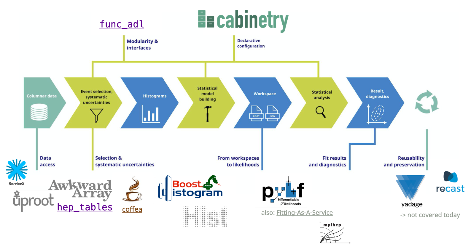
Tools and packages used in this example#
The notebook showcases: - data delivery with ServiceX - event / column selection with func_adl - data handling with awkward-array - histogram production with coffea - histogram handling with hist - visualization with mplhep, hist & matplotlib - ROOT file handling with uproot - statistical model construction with cabinetry - statistical inference with pyhf
High-level strategy#
We will define which files to process, set up a query with func_adl to extract data provided by ServiceX, and use coffea to construct histograms. Those histograms will be saved with uproot, and then assembled into a statistical model with cabinetry. Following that, we perform statistical inference with pyhf.
Required setup for this notebook#
If you are running on the coffea-casa Open Data instance, ServiceX credentials are automatically available to you. Otherwise you will need to set those up. Create a file servicex.yaml in your home directory, or the place this notebook is located in.
See this talk by KyungEon and the ServiceX doc for more information.
Files to process#
To get started, we define which files are going to be processed in this notebook. We also set some information for histogramming that will be used subsequently.
[3]:
prefix = (
    "http://xrootd-local.unl.edu:1094//store/user/AGC/ATLAS_HZZ/"
)

# labels for combinations of datasets
z_ttbar = r"Background $Z,t\bar{t}$"
zzstar = r"Background $ZZ^{\star}$"
signal = r"Signal ($m_H$ = 125 GeV)"

input_files = {
    "Data": [
        prefix + "data_A.4lep.root",
        prefix + "data_B.4lep.root",
        prefix + "data_C.4lep.root",
        prefix + "data_D.4lep.root",
    ],
    z_ttbar: [
        prefix + "mc_361106.Zee.4lep.root",
        prefix + "mc_361107.Zmumu.4lep.root",
        prefix + "mc_410000.ttbar_lep.4lep.root",
    ],
    zzstar: [prefix + "mc_363490.llll.4lep.root"],
    signal: [
        prefix + "mc_345060.ggH125_ZZ4lep.4lep.root",
        prefix + "mc_344235.VBFH125_ZZ4lep.4lep.root",
        prefix + "mc_341964.WH125_ZZ4lep.4lep.root",
        prefix + "mc_341947.ZH125_ZZ4lep.4lep.root",
    ],
}

# information for histograms
bin_edge_low = 80  # 80 GeV
bin_edge_high = 250  # 250 GeV
num_bins = 34
Setting up a query with func_adl#
We are using func_adl for event & column selection, and make a datasource with the query built by get_lepton_query.
A list of all available columns in the input files can be found in the ATLAS documentation of branches.
Systematic uncertainty added: scale factor variation, applied already at event selection stage. Imagine that this could be a calculation that requires a lot of different variables which are no longer needed downstream afterwards, so it makes sense to do it here.
[4]:
def get_lepton_query():
    """Performs event selection with func_adl transformer: require events with exactly four leptons.
    Also select all columns needed further downstream for processing &
    histogram filling.
    """
    from servicex import query as q
    return q.FuncADL_Uproot().FromTree('mini')\
        .Where(lambda event: event.lep_n == 4).Select(
        lambda e: {
            "lep_pt": e.lep_pt,
            "lep_eta": e.lep_eta,
            "lep_phi": e.lep_phi,
            "lep_energy": e.lep_E,
            "lep_charge": e.lep_charge,
            "lep_typeid": e.lep_type,
            "mcWeight": e.mcWeight,
            "scaleFactor": e.scaleFactor_ELE
            * e.scaleFactor_MUON
            * e.scaleFactor_LepTRIGGER
            * e.scaleFactor_PILEUP,
            # scale factor systematic variation example
            "scaleFactorUP": e.scaleFactor_ELE
            * e.scaleFactor_MUON
            * e.scaleFactor_LepTRIGGER
            * e.scaleFactor_PILEUP
            * 1.1,
            "scaleFactorDOWN": e.scaleFactor_ELE
            * e.scaleFactor_MUON
            * e.scaleFactor_LepTRIGGER
            * e.scaleFactor_PILEUP
            * 0.9,
        }
    )

def get_lepton_query_uproot_raw():
    """Performs event selection with uproot-raw transformer: require events with exactly four leptons.
    Also select all columns needed further downstream for processing &
    histogram filling.
    """
    from servicex import query as q
    return q.UprootRaw([{'treename': 'mini',
                         'expressions': ['lep_pt', 'lep_eta', 'lep_phi', 'lep_energy', 'lep_charge',
                                         'lep_typeid', 'mcWeight', 'scaleFactor', 'scaleFactorUP', 'scaleFactorDOWN'],
                         'aliases': { 'lep_typeid': 'lep_type', 'lep_energy': 'lep_E',
                                      'scaleFactor': 'scaleFactor_ELE*scaleFactor_MUON*scaleFactor_LepTRIGGER*scaleFactor_PILEUP',
                                      'scaleFactorUP': 'scaleFactor*1.1',
                                      'scaleFactorDOWN': 'scaleFactor*0.9' }
                        }])
Caching the queried datasets with ServiceX#
Using the queries created with func_adl, we are using ServiceX to read the ATLAS Open Data files to build cached files with only the specific event information as dictated by the query.
[5]:
# create the query
if USE_SERVICEX_UPROOT_RAW:
    query = get_lepton_query_uproot_raw()
else:
    query = get_lepton_query()

# now we query the files and create a fileset dictionary containing the
# URLs pointing to the queried files

t0 = time.time()

fileset = {}

bundle = { 'General': { 'Delivery': 'URLs' },
           'Sample': [ { 'Name': ds_name,
                          'Query': query,
                          'Dataset': servicex.dataset.FileList(input_files[ds_name]),
                          'IgnoreLocalCache': IGNORE_CACHE } for ds_name in input_files.keys() ]
           }

results = servicex.deliver(bundle)
fileset = { _: {"files": results[_], "metadata": {"dataset_name": _}} for _ in results }

print(f"execution took {time.time() - t0:.2f} seconds")
execution took 31.85 seconds
We now have a fileset dictionary containing the addresses of the queried files, ready to pass to coffea:
[6]:
fileset
[6]:
{'Data': {'files': ['http://s3v2.af.uchicago.edu:32095/2aaf4d87-f4a4-43e1-87d5-18ceb084a73e/root%3A%3A%3Axcache.af.uchicago.edu%3A%3Ahttp%3A%3A%3Axrootd-local.unl.edu%3A1094%3A%3Astore%3Auser%3AAGC%3AATLAS_HZZ%3Adata_A.4lep.root?X-Amz-Algorithm=AWS4-HMAC-SHA256&X-Amz-Credential=ABAOJZ4XMLKWO5H0PZJ3%2F20241003%2Faf-object-store%2Fs3%2Faws4_request&X-Amz-Date=20241003T063422Z&X-Amz-Expires=604800&X-Amz-SignedHeaders=host&X-Amz-Signature=5563bf77a381e1d7d76ad67c65807d1eb0e9793e37edd8389fdea23b3c490da5', 'http://s3v2.af.uchicago.edu:32095/2aaf4d87-f4a4-43e1-87d5-18ceb084a73e/root%3A%3A%3Axcache.af.uchicago.edu%3A%3Ahttp%3A%3A%3Axrootd-local.unl.edu%3A1094%3A%3Astore%3Auser%3AAGC%3AATLAS_HZZ%3Adata_B.4lep.root?X-Amz-Algorithm=AWS4-HMAC-SHA256&X-Amz-Credential=ABAOJZ4XMLKWO5H0PZJ3%2F20241003%2Faf-object-store%2Fs3%2Faws4_request&X-Amz-Date=20241003T063427Z&X-Amz-Expires=604800&X-Amz-SignedHeaders=host&X-Amz-Signature=55df5b734512deb29b4dcaa8715baf9fdbee4d6dbe9140abb9803c66a26afbe4', 'http://s3v2.af.uchicago.edu:32095/2aaf4d87-f4a4-43e1-87d5-18ceb084a73e/root%3A%3A%3Axcache.af.uchicago.edu%3A%3Ahttp%3A%3A%3Axrootd-local.unl.edu%3A1094%3A%3Astore%3Auser%3AAGC%3AATLAS_HZZ%3Adata_C.4lep.root?X-Amz-Algorithm=AWS4-HMAC-SHA256&X-Amz-Credential=ABAOJZ4XMLKWO5H0PZJ3%2F20241003%2Faf-object-store%2Fs3%2Faws4_request&X-Amz-Date=20241003T063427Z&X-Amz-Expires=604800&X-Amz-SignedHeaders=host&X-Amz-Signature=3efbd4716e4311d3bdc6bb75d8d5f12e5fff835018caf5221c89cc9e5975157b', 'http://s3v2.af.uchicago.edu:32095/2aaf4d87-f4a4-43e1-87d5-18ceb084a73e/root%3A%3A%3Axcache.af.uchicago.edu%3A%3Ahttp%3A%3A%3Axrootd-local.unl.edu%3A1094%3A%3Astore%3Auser%3AAGC%3AATLAS_HZZ%3Adata_D.4lep.root?X-Amz-Algorithm=AWS4-HMAC-SHA256&X-Amz-Credential=ABAOJZ4XMLKWO5H0PZJ3%2F20241003%2Faf-object-store%2Fs3%2Faws4_request&X-Amz-Date=20241003T063427Z&X-Amz-Expires=604800&X-Amz-SignedHeaders=host&X-Amz-Signature=169efaa840d75a6b04b1140c77e61a8b044373ce4abcdb4a1d6233b8942cf84a'],
  'metadata': {'dataset_name': 'Data'}},
 'Background $Z,t\\bar{t}$': {'files': ['http://s3v2.af.uchicago.edu:32095/69ec4b48-f001-4d63-9bac-2c4e1c560728/root%3A%3A%3Axcache.af.uchicago.edu%3A%3Ahttp%3A%3A%3Axrootd-local.unl.edu%3A1094%3A%3Astore%3Auser%3AAGC%3AATLAS_HZZ%3Amc_361106.Zee.4lep.root?X-Amz-Algorithm=AWS4-HMAC-SHA256&X-Amz-Credential=ABAOJZ4XMLKWO5H0PZJ3%2F20241003%2Faf-object-store%2Fs3%2Faws4_request&X-Amz-Date=20241003T063427Z&X-Amz-Expires=604800&X-Amz-SignedHeaders=host&X-Amz-Signature=ef20fcb47afcb1f5dc89867d0d55c97aafa5bfd7fd5a116fe05c3b5b06e44273', 'http://s3v2.af.uchicago.edu:32095/69ec4b48-f001-4d63-9bac-2c4e1c560728/root%3A%3A%3Axcache.af.uchicago.edu%3A%3Ahttp%3A%3A%3Axrootd-local.unl.edu%3A1094%3A%3Astore%3Auser%3AAGC%3AATLAS_HZZ%3Amc_361107.Zmumu.4lep.root?X-Amz-Algorithm=AWS4-HMAC-SHA256&X-Amz-Credential=ABAOJZ4XMLKWO5H0PZJ3%2F20241003%2Faf-object-store%2Fs3%2Faws4_request&X-Amz-Date=20241003T063432Z&X-Amz-Expires=604800&X-Amz-SignedHeaders=host&X-Amz-Signature=46b1aeb2f4498d9134aeeb4c2fac4bc19872613ba523490bad1a316bbd50dff2', 'http://s3v2.af.uchicago.edu:32095/69ec4b48-f001-4d63-9bac-2c4e1c560728/root%3A%3A%3Axcache.af.uchicago.edu%3A%3Ahttp%3A%3A%3Axrootd-local.unl.edu%3A1094%3A%3Astore%3Auser%3AAGC%3AATLAS_HZZ%3Amc_410000.ttbar_lep.4lep.root?X-Amz-Algorithm=AWS4-HMAC-SHA256&X-Amz-Credential=ABAOJZ4XMLKWO5H0PZJ3%2F20241003%2Faf-object-store%2Fs3%2Faws4_request&X-Amz-Date=20241003T063437Z&X-Amz-Expires=604800&X-Amz-SignedHeaders=host&X-Amz-Signature=8ed564063e68075229e6f19844e793d0db3b79b7edc29ebea62c29f10228fe11'],
  'metadata': {'dataset_name': 'Background $Z,t\\bar{t}$'}},
 'Background $ZZ^{\\star}$': {'files': ['http://s3v2.af.uchicago.edu:32095/1d45f18f-c647-4e34-ad5e-1a994ebe7500/root%3A%3A%3Axcache.af.uchicago.edu%3A%3Ahttp%3A%3A%3Axrootd-local.unl.edu%3A1094%3A%3Astore%3Auser%3AAGC%3AATLAS_HZZ%3Amc_363490.llll.4lep.root?X-Amz-Algorithm=AWS4-HMAC-SHA256&X-Amz-Credential=ABAOJZ4XMLKWO5H0PZJ3%2F20241003%2Faf-object-store%2Fs3%2Faws4_request&X-Amz-Date=20241003T063427Z&X-Amz-Expires=604800&X-Amz-SignedHeaders=host&X-Amz-Signature=0ef85def5136da437133412e67dc018173bfcee2ca8e16b63d5ba949d789d923'],
  'metadata': {'dataset_name': 'Background $ZZ^{\\star}$'}},
 'Signal ($m_H$ = 125 GeV)': {'files': ['http://s3v2.af.uchicago.edu:32095/43016873-3dbb-47f9-847f-3ab3a81133fa/root%3A%3A%3Axcache.af.uchicago.edu%3A%3Ahttp%3A%3A%3Axrootd-local.unl.edu%3A1094%3A%3Astore%3Auser%3AAGC%3AATLAS_HZZ%3Amc_341947.ZH125_ZZ4lep.4lep.root?X-Amz-Algorithm=AWS4-HMAC-SHA256&X-Amz-Credential=ABAOJZ4XMLKWO5H0PZJ3%2F20241003%2Faf-object-store%2Fs3%2Faws4_request&X-Amz-Date=20241003T063427Z&X-Amz-Expires=604800&X-Amz-SignedHeaders=host&X-Amz-Signature=7c838ff2eadb32f0b013d9bc48d5cd7764c0eb08407175ff1ea8d6c29b259d2d', 'http://s3v2.af.uchicago.edu:32095/43016873-3dbb-47f9-847f-3ab3a81133fa/root%3A%3A%3Axcache.af.uchicago.edu%3A%3Ahttp%3A%3A%3Axrootd-local.unl.edu%3A1094%3A%3Astore%3Auser%3AAGC%3AATLAS_HZZ%3Amc_341964.WH125_ZZ4lep.4lep.root?X-Amz-Algorithm=AWS4-HMAC-SHA256&X-Amz-Credential=ABAOJZ4XMLKWO5H0PZJ3%2F20241003%2Faf-object-store%2Fs3%2Faws4_request&X-Amz-Date=20241003T063427Z&X-Amz-Expires=604800&X-Amz-SignedHeaders=host&X-Amz-Signature=7e7e74cb2175d8c533ea9ed73a17bb07160d7152c1600290e7272ba4444a8859', 'http://s3v2.af.uchicago.edu:32095/43016873-3dbb-47f9-847f-3ab3a81133fa/root%3A%3A%3Axcache.af.uchicago.edu%3A%3Ahttp%3A%3A%3Axrootd-local.unl.edu%3A1094%3A%3Astore%3Auser%3AAGC%3AATLAS_HZZ%3Amc_344235.VBFH125_ZZ4lep.4lep.root?X-Amz-Algorithm=AWS4-HMAC-SHA256&X-Amz-Credential=ABAOJZ4XMLKWO5H0PZJ3%2F20241003%2Faf-object-store%2Fs3%2Faws4_request&X-Amz-Date=20241003T063427Z&X-Amz-Expires=604800&X-Amz-SignedHeaders=host&X-Amz-Signature=6fb165b3da4d4346f2ac7f5e92b8d9df08c8208ec241b9102eec0626921d32e3', 'http://s3v2.af.uchicago.edu:32095/43016873-3dbb-47f9-847f-3ab3a81133fa/root%3A%3A%3Axcache.af.uchicago.edu%3A%3Ahttp%3A%3A%3Axrootd-local.unl.edu%3A1094%3A%3Astore%3Auser%3AAGC%3AATLAS_HZZ%3Amc_345060.ggH125_ZZ4lep.4lep.root?X-Amz-Algorithm=AWS4-HMAC-SHA256&X-Amz-Credential=ABAOJZ4XMLKWO5H0PZJ3%2F20241003%2Faf-object-store%2Fs3%2Faws4_request&X-Amz-Date=20241003T063427Z&X-Amz-Expires=604800&X-Amz-SignedHeaders=host&X-Amz-Signature=583b5bc164f2a0ead7fc825ff53c9266d2ef7379f03ab006cf17aff2ed0f3c97'],
  'metadata': {'dataset_name': 'Signal ($m_H$ = 125 GeV)'}}}
Processing ServiceX-provided data with coffea#
Event weighting: look up cross-section from a provided utility file, and correctly normalize all events.
[7]:
def get_xsec_weight(sample: str) -> float:
    """Returns normalization weight for a given sample."""
    lumi = 10_000  # pb^-1
    xsec_map = infofile.infos[sample]  # dictionary with event weighting information
    xsec_weight = (lumi * xsec_map["xsec"]) / (xsec_map["sumw"] * xsec_map["red_eff"])
    return xsec_weight
Cuts to apply: - two opposite flavor lepton pairs (total lepton charge is 0) - lepton types: 4 electrons, 4 muons, or 2 electrons + 2 muons
[8]:
def lepton_filter(lep_charge, lep_type):
    """Filters leptons: sum of charges is required to be 0, and sum of lepton types 44/48/52.
    Electrons have type 11, muons have 13, so this means 4e/4mu/2e2mu.
    """
    sum_lep_charge = ak.sum(lep_charge, axis=1)
    sum_lep_type = ak.sum(lep_type, axis=1)
    good_lep_type = ak.any(
        [sum_lep_type == 44, sum_lep_type == 48, sum_lep_type == 52], axis=0
    )
    return ak.all([sum_lep_charge == 0, good_lep_type], axis=0)
Set up the coffea processor. It will apply cuts, calculate the four-lepton invariant mass, and fill a histogram.
Systematic uncertainty added: m4l variation, applied in the processor to remaining events. This might instead for example be the result of applying a tool performing a computationally expensive calculation, which should only be run for events where it is needed.
[9]:
class HZZAnalysis(processor.ProcessorABC):
    """The coffea processor used in this analysis."""

    def __init__(self):
        pass

    def process(self, events):
        vector.register_awkward()
        # type of dataset being processed, provided via metadata (comes originally from fileset)
        dataset_category = events.metadata["dataset_name"]

        # apply a cut to events, based on lepton charge and lepton type
        events = events[lepton_filter(events.lep_charge, events.lep_typeid)]

        # construct lepton four-vectors
        leptons = ak.zip(
            {"pt": events.lep_pt,
             "eta": events.lep_eta,
             "phi": events.lep_phi,
             "energy": events.lep_energy},
            with_name="Momentum4D",
        )

        # calculate the 4-lepton invariant mass for each remaining event
        # this could also be an expensive calculation using external tools
        mllll = (
            leptons[:, 0] + leptons[:, 1] + leptons[:, 2] + leptons[:, 3]
        ).mass / 1000

        # creat histogram holding outputs, for data just binned in m4l
        mllllhist_data = hist.Hist.new.Reg(
            num_bins,
            bin_edge_low,
            bin_edge_high,
            name="mllll",
            label="$\mathrm{m_{4l}}$ [GeV]",
        ).Weight()  # using weighted storage here for plotting later, but not needed

        # three histogram axes for MC: m4l, category, and variation (nominal and
        # systematic variations)
        mllllhist_MC = (
            hist.Hist.new.Reg(
                num_bins,
                bin_edge_low,
                bin_edge_high,
                name="mllll",
                label="$\mathrm{m_{4l}}$ [GeV]",
            )
            .StrCat([k for k in fileset.keys() if k != "Data"], name="dataset")
            .StrCat(
                ["nominal", "scaleFactorUP", "scaleFactorDOWN", "m4lUP", "m4lDOWN"],
                name="variation",
            )
            .Weight()
        )

        if dataset_category == "Data":
            # create and fill a histogram for m4l
            mllllhist_data.fill(mllll=mllll)

        else:
            # extract the sample name from the filename to calculate x-sec weight
            sample = re.findall(r"mc_\d+\.(.+)\.4lep", events.metadata["filename"])[0]
            basic_weight = get_xsec_weight(sample) * events.mcWeight
            totalWeights = basic_weight * events.scaleFactor

            # calculate systematic variations for weight
            totalWeightsUp = basic_weight * events.scaleFactorUP
            totalWeightsDown = basic_weight * events.scaleFactorDOWN

            # create and fill weighted histograms for m4l: nominal and variations
            mllllhist_MC.fill(
                mllll=mllll,
                dataset=dataset_category,
                variation="nominal",
                weight=totalWeights,
            )

            # scale factor variations
            mllllhist_MC.fill(
                mllll=mllll,
                dataset=dataset_category,
                variation="scaleFactorUP",
                weight=totalWeightsUp,
            )
            mllllhist_MC.fill(
                mllll=mllll,
                dataset=dataset_category,
                variation="scaleFactorDOWN",
                weight=totalWeightsDown,
            )

            # variation in 4-lepton invariant mass
            mllllhist_MC.fill(
                mllll=mllll * 1.01,
                dataset=dataset_category,
                variation="m4lUP",
                weight=totalWeights,
            )
            mllllhist_MC.fill(
                mllll=mllll * 0.99,
                dataset=dataset_category,
                variation="m4lDOWN",
                weight=totalWeights,
            )

        return {"data": mllllhist_data, "MC": mllllhist_MC}

    def postprocess(self, accumulator):
        pass
Producing the desired histograms#
Run the processor on data previously gathered by ServiceX, then gather output histograms.
[10]:
t0 = time.time()

executor = processor.FuturesExecutor(workers=NUM_CORES)
run = processor.Runner(executor=executor, savemetrics=True, metadata_cache={},
                       chunksize=CHUNKSIZE, schema=BaseSchema)
# The trees returned by ServiceX will have different names depending on the query language used
all_histograms, metrics = run(fileset, "mini" if USE_SERVICEX_UPROOT_RAW else "servicex", processor_instance=HZZAnalysis())

print(f"execution took {time.time() - t0:.2f} seconds")
execution took 25.43 seconds
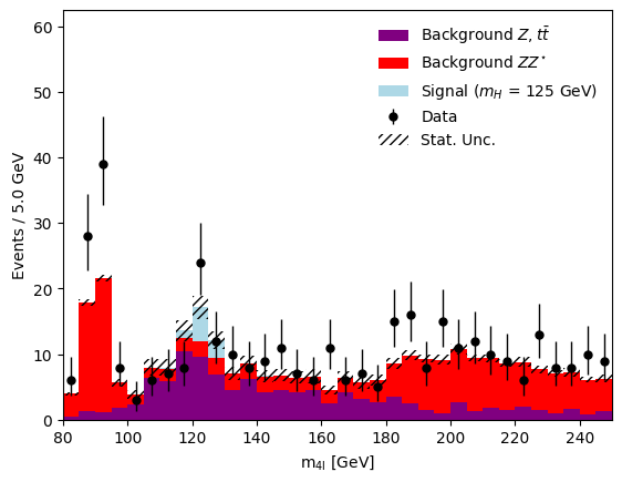
Plotting histograms with mplhep, hist & matplotlib#
We can plot some of the histograms we just produced with mplhep, hist & matplotlib.
[11]:
# plot histograms with mplhep & hist
mplhep.histplot(
    all_histograms["data"], histtype="errorbar", color="black", label="Data"
)
hist.Hist.plot1d(
    all_histograms["MC"][:, :, "nominal"],
    stack=True,
    histtype="fill",
    color=["purple", "red", "lightblue"],
)

# plot band for MC statistical uncertainties via utility function
# (this uses matplotlib directly)
utils.plot_errorband(bin_edge_low, bin_edge_high, num_bins, all_histograms)

# we are using a small utility function to also save the figure in .png and .pdf
# format, you can find the produced figure in the figures/ folder
utils.save_figure("m4l_stat_uncertainty")
Saving histograms with uproot#
In order to build a statistical model, we will use cabinetry’s support for reading histograms to build a so-called workspace specifying the model. We will save the histograms we just created to disk with uproot.
[12]:
file_name = "histograms.root"
with uproot.recreate(file_name) as f:
    f["data"] = all_histograms["data"]

    f["Z_tt"] = all_histograms["MC"][:, z_ttbar, "nominal"]
    f["Z_tt_SF_up"] = all_histograms["MC"][:, z_ttbar, "scaleFactorUP"]
    f["Z_tt_SF_down"] = all_histograms["MC"][:, z_ttbar, "scaleFactorDOWN"]
    f["Z_tt_m4l_up"] = all_histograms["MC"][:, z_ttbar, "m4lUP"]
    f["Z_tt_m4l_down"] = all_histograms["MC"][:, z_ttbar, "m4lDOWN"]

    f["ZZ"] = all_histograms["MC"][:, zzstar, "nominal"]
    f["ZZ_SF_up"] = all_histograms["MC"][:, zzstar, "scaleFactorUP"]
    f["ZZ_SF_down"] = all_histograms["MC"][:, zzstar, "scaleFactorDOWN"]
    f["ZZ_m4l_up"] = all_histograms["MC"][:, zzstar, "m4lUP"]
    f["ZZ_m4l_down"] = all_histograms["MC"][:, zzstar, "m4lDOWN"]

    f["signal"] = all_histograms["MC"][:, signal, "nominal"]
    f["signal_SF_up"] = all_histograms["MC"][:, signal, "scaleFactorUP"]
    f["signal_SF_down"] = all_histograms["MC"][:, signal, "scaleFactorDOWN"]
    f["signal_m4l_up"] = all_histograms["MC"][:, signal, "m4lUP"]
    f["signal_m4l_down"] = all_histograms["MC"][:, signal, "m4lDOWN"]
Building a workspace and running a fit with cabinetry & pyhf#
Take a look at the cabinetry configuration file in config.yml. It specifies the model to be built. In particular, it lists the samples we are going to be using:
[13]:
config = cabinetry.configuration.load("config.yml")
config["Samples"]
INFO - cabinetry.configuration - opening config file config.yml
[13]:
[{'Name': 'Data', 'SamplePath': 'data', 'Data': True},
 {'Name': 'Signal', 'SamplePath': 'signal'},
 {'Name': 'Background ZZ*', 'SamplePath': 'ZZ'},
 {'Name': 'Background Z, ttbar', 'SamplePath': 'Z_tt'}]
It also shows which systematic uncertainties we will apply. This includes a new systematic uncertainty defined at this stage.
Systematic uncertainty added: \(ZZ^\star\) normalization; this does not require any histograms, so we can define it here.
[14]:
config["Systematics"]
[14]:
[{'Name': 'Scalefactor_variation',
  'Type': 'NormPlusShape',
  'Up': {'VariationPath': '_SF_up'},
  'Down': {'VariationPath': '_SF_down'}},
 {'Name': 'm4l_variation',
  'Type': 'NormPlusShape',
  'Up': {'VariationPath': '_m4l_up'},
  'Down': {'VariationPath': '_m4l_down'}},
 {'Name': 'ZZ_norm',
  'Type': 'Normalization',
  'Up': {'Normalization': 0.1},
  'Down': {'Normalization': -0.1},
  'Samples': 'Background ZZ*'}]
The information in the configuration is used to construct a statistical model, the workspace.
[15]:
cabinetry.templates.collect(config)
cabinetry.templates.postprocess(config)  # optional post-processing (e.g. smoothing)
ws = cabinetry.workspace.build(config)
INFO - cabinetry.workspace - building workspace
Create a pyhf model and extract the data from the workspace. Perform a MLE fit, the results will be reported in the output.
[16]:
model, data = cabinetry.model_utils.model_and_data(ws)
fit_results = cabinetry.fit.fit(model, data)
INFO - cabinetry.fit - performing maximum likelihood fit
INFO - cabinetry.fit - Migrad status:
┌─────────────────────────────────────────────────────────────────────────┐
│                                Migrad                                   │
├──────────────────────────────────┬──────────────────────────────────────┤
│ FCN = 82.52                      │             Nfcn = 2400              │
│ EDM = 3.3e-10 (Goal: 0.0002)     │                                      │
├──────────────────────────────────┼──────────────────────────────────────┤
│          Valid Minimum           │        No Parameters at limit        │
├──────────────────────────────────┼──────────────────────────────────────┤
│ Below EDM threshold (goal x 10)  │           Below call limit           │
├───────────────┬──────────────────┼───────────┬─────────────┬────────────┤
│  Covariance   │     Hesse ok     │ Accurate  │  Pos. def.  │ Not forced │
└───────────────┴──────────────────┴───────────┴─────────────┴────────────┘
INFO - cabinetry.fit - fit results (with symmetric uncertainties):
INFO - cabinetry.fit - Scalefactor_variation       =  1.1483 +/- 0.6706
INFO - cabinetry.fit - m4l_variation               =  0.1614 +/- 0.5158
INFO - cabinetry.fit - Signal_norm                 =  1.1207 +/- 0.7096
INFO - cabinetry.fit - ZZ_norm                     =  1.5474 +/- 0.8128
INFO - cabinetry.fit - staterror_Signal_region[0]  =  1.0037 +/- 0.0583
INFO - cabinetry.fit - staterror_Signal_region[1]  =  1.0038 +/- 0.0253
INFO - cabinetry.fit - staterror_Signal_region[2]  =  1.0059 +/- 0.0237
INFO - cabinetry.fit - staterror_Signal_region[3]  =  1.0074 +/- 0.1028
INFO - cabinetry.fit - staterror_Signal_region[4]  =  0.9558 +/- 0.1658
INFO - cabinetry.fit - staterror_Signal_region[5]  =  0.9330 +/- 0.1489
INFO - cabinetry.fit - staterror_Signal_region[6]  =  0.9528 +/- 0.1427
INFO - cabinetry.fit - staterror_Signal_region[7]  =  0.9109 +/- 0.1100
INFO - cabinetry.fit - staterror_Signal_region[8]  =  1.0446 +/- 0.0987
INFO - cabinetry.fit - staterror_Signal_region[9]  =  0.9559 +/- 0.1092
INFO - cabinetry.fit - staterror_Signal_region[10] =  1.0264 +/- 0.1266
INFO - cabinetry.fit - staterror_Signal_region[11] =  0.9630 +/- 0.1329
INFO - cabinetry.fit - staterror_Signal_region[12] =  1.0218 +/- 0.1343
INFO - cabinetry.fit - staterror_Signal_region[13] =  1.0480 +/- 0.1293
INFO - cabinetry.fit - staterror_Signal_region[14] =  0.9919 +/- 0.1325
INFO - cabinetry.fit - staterror_Signal_region[15] =  0.9582 +/- 0.1510
INFO - cabinetry.fit - staterror_Signal_region[16] =  1.0992 +/- 0.1349
INFO - cabinetry.fit - staterror_Signal_region[17] =  0.9597 +/- 0.1563
INFO - cabinetry.fit - staterror_Signal_region[18] =  1.0102 +/- 0.1482
INFO - cabinetry.fit - staterror_Signal_region[19] =  0.9570 +/- 0.1359
INFO - cabinetry.fit - staterror_Signal_region[20] =  1.0406 +/- 0.0930
INFO - cabinetry.fit - staterror_Signal_region[21] =  1.0219 +/- 0.0761
INFO - cabinetry.fit - staterror_Signal_region[22] =  0.9867 +/- 0.0592
INFO - cabinetry.fit - staterror_Signal_region[23] =  1.0184 +/- 0.0750
INFO - cabinetry.fit - staterror_Signal_region[24] =  0.9878 +/- 0.0719
INFO - cabinetry.fit - staterror_Signal_region[25] =  1.0000 +/- 0.0575
INFO - cabinetry.fit - staterror_Signal_region[26] =  0.9918 +/- 0.0666
INFO - cabinetry.fit - staterror_Signal_region[27] =  0.9917 +/- 0.0656
INFO - cabinetry.fit - staterror_Signal_region[28] =  0.9640 +/- 0.0863
INFO - cabinetry.fit - staterror_Signal_region[29] =  1.0202 +/- 0.0812
INFO - cabinetry.fit - staterror_Signal_region[30] =  0.9955 +/- 0.0712
INFO - cabinetry.fit - staterror_Signal_region[31] =  0.9907 +/- 0.0915
INFO - cabinetry.fit - staterror_Signal_region[32] =  1.0110 +/- 0.0690
INFO - cabinetry.fit - staterror_Signal_region[33] =  1.0092 +/- 0.0903
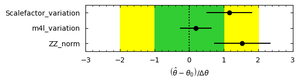
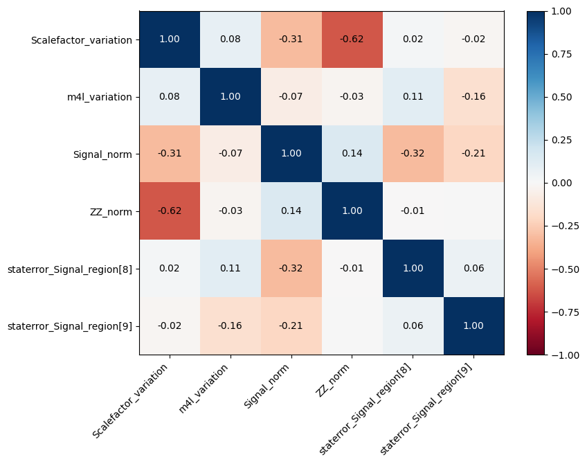
We can visualize the pulls and correlations. cabinetry saves this figure by default as a .pdf, but here we will use our small utility again to save in both .png and .pdf format.
[17]:
cabinetry.visualize.pulls(
    fit_results, exclude="Signal_norm", close_figure=False, save_figure=False
)
utils.save_figure("pulls")
[18]:
cabinetry.visualize.correlation_matrix(
    fit_results, pruning_threshold=0.15, close_figure=False, save_figure=False
)
utils.save_figure("correlation_matrix")
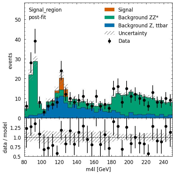
Finally, visualize the post-fit model and data. We first create the post-fit model prediction, using the model and the best-fit resuts.
The visualization is using information stored in the workspace, which does not include binning or which observable is used. This information can be passed in via the config kwarg, but we can also edit the figure after its creation. We will demonstrate both approaches below.
[19]:
# create post-fit model prediction
postfit_model = cabinetry.model_utils.prediction(model, fit_results=fit_results)

# binning to use in plot
plot_config = {
    "Regions": [
        {
            "Name": "Signal_region",
            "Binning": list(np.linspace(bin_edge_low, bin_edge_high, num_bins + 1)),
        }
    ]
}

figure_dict = cabinetry.visualize.data_mc(
    postfit_model, data, config=plot_config, save_figure=False
)

# modify x-axis label
fig = figure_dict[0]["figure"]
fig.axes[1].set_xlabel("m4l [GeV]")

# let's also save the figure
utils.save_figure("Signal_region_postfit")
We can also use pyhf directly. We already have a model and data, so let’s calculate the CLs value.
[20]:
mu_test = 1.0
cls = float(pyhf.infer.hypotest(mu_test, data, model))
print(f"CL_S for Signal_norm={mu_test} is {cls:.3f}")
CL_S for Signal_norm=1.0 is 0.534
Final remarks: control flow and duplication of information#
In the demonstration today we first built histograms, making sure we produce all that we will need for our statistical model. We then built the model, saying where to find each histogram. If we want to add a new histogram-based systematic uncertainty, we will need to implement it in two places: - in the histogram-producing code (e.g. coffea processor), - in the model building instructions.
It can be convenient to avoid this duplication, which can be achieved as follows: - specify all relevant information in the model building configuration, - use that information to steer the histogram production.
This method is available in cabinetry, check out the cabinetry tutorials repository to see it in action. With this approach cabinetry builds the histograms it needs itself.
This works well for some cases, but not for others: - a simple cut can be specified easily in the configuration, and varied for systematic uncertainties, - a complex calculation cannot easily be captured in such a way.
The image below describes different options. The general considerations here are independent of the exact tools used, and should apply equally when using similar workflows.
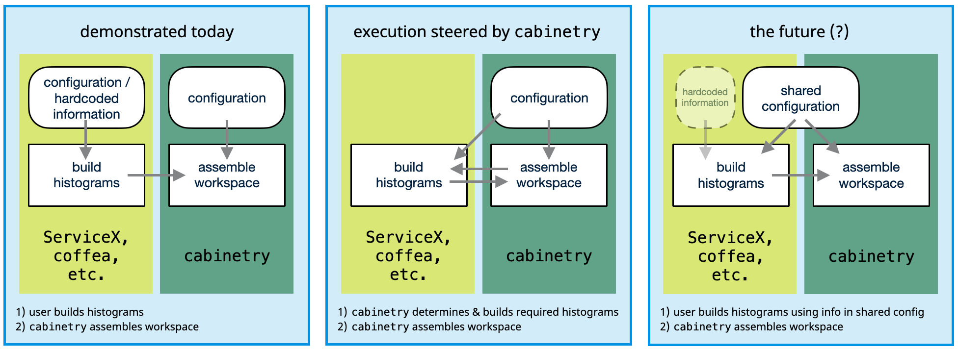
A flexible design that works well for all scenarios is needed here, but is not available yet. If you have thoughts about this, please do get in touch!
Exercises#
Here are a few ideas to try out to become more familiar with the tools shown in this notebook:
Run the notebook a second time. It should be faster now — you are taking advantage of caching!
Change the event pre-selection in the
func_adlquery. Try out requiring exactly zero jets. Has the analysis become more or less sensitive after this change?Change the lepton requirements. What happens when only accepting events with 4 electrons or 4 muons?
Try a different binning. Note how you still benefit from caching in the
ServiceX-delivered data!Compare the pre- and post-fit data/MC agreement (hint: the
fit_resultskwarg incabinetry.model_utils.predictionis optional).Find the value of the
Signal_normnormalization factor for which CL_S = 0.05, the 95% confidence level upper parameter limit (hint: usepyhfdirectly, orcabinetry.fit.limit).Separate the \(Z\) and \(t\bar{t}\) backgrounds and add a 6% normalization uncertainty for \(t\bar{t}\) in the fit.
Replace the 10% normalization uncertainty for the \(ZZ^\star\) background by a free-floating normalization factor in the fit.
Advanced ideas: - Implement a more realistic systematic uncertainty in the coffea processor, for example for detector-related uncertainties for lepton kinematics. Propagate it through the analysis chain to observe the impact in a ranking plot produced with cabinetry. - Try out this workflow with your own analysis! Are there missing features or ways to streamline the experience? If so, please let us know!